Lorentz Attractor

Introduction

Lorenz system [1] is one of the well studied non-linear model in system dynamics. Even though being well explored and simulated, it is a beautiful simplistic system that showcase chaotic behaviour for particular set of initial conditions. The non-linear differential equations were initially studied by N. Lorenz, a meteorologist during 1963.

$$ \tag{1} \frac {dx}{dt} = \sigma (y - x) $$ $$ \tag{2} \frac {dy}{dt} = x(\rho -z ) - y $$ $$ \tag{3} \frac {dz}{dt} = xy - \beta z $$

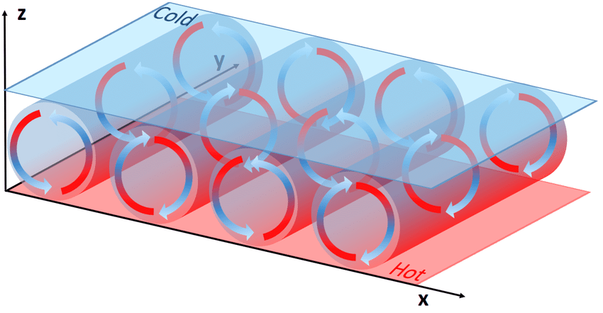
The equation (1), (2) and (3) are simplified form of heat convection in earth atmosphere which is governed by the famous Navier-stokes equation. These equations could help to model and understand natural heat convection in fluid dynamics. Heat convection is the physical process where transfer of heat occurs due to movement of the fluid. Figure 1 shows a typical experimental setup for understanding heat convection. It consist of fluid between two parallel plates. When the bottom plate is exposed to hot temperature and top plate to ambient room temperature, this creates a linear heat gradient between the two plates. The hot fluid near the bottom plate is less dense, compared to cold fluid on top. This difference in the density, causes the cold fluid to move down towards the bottom due to gravity and the hot fluid to raise up. A continous cycle of the fluid movement is established, creating a cell like structure in between the parallel plates called convection cells as depicted in Figure 1. This pattern of convection cells are also called Rayleigh-Bernad convection cells, named after Lord Rayleigh, who sucessfully analyzed the structure in 1916.
 

Simulation

Parameters

These equations govern the temporal evolution of three physical quantities, namely $ x $ corresponds to the rate of convection happening between the two plate. $y$ corresponds to the horizontal temperature variation and $ z $ corresponds to the vertical temperature variation. $ \sigma, \rho $ and $ \beta $ are constants of the system. The system is highly sensitive to initial conditions ($\sigma , \rho $ and $\beta$) that we choose. Starting the simulation with a different values of $ \sigma, \rho $ or $\beta $ that are infinitesimally different from each other could create a completely different output. In the following blog, the implementation and simulation of the equation in python is discussed along with visualization. Further, the behaviour of the system is analysed for different values of $ \sigma, \rho $ and $ \beta $ in the next blog post.

Implementation

Python scipy library has a powerful ODE solver to simulate these equation. Even though the ODE solvers are quiet good, using a basic numerical itegration like Runge-Kutta 4 method gives a better understading of simulation ODE’s.

import numpy as np
x0 = [1, 1, 1]  # quantities vector [x,y,z]
sigma=10.0 
beta=8.0/3 
rho=28.0
t = np.linspace(0, 3, 1000)  # time vector 

The fourth order Runge-Kutta method also known as RK4, is an implicit-explicit iterative numerical integration method that includes the first order Euler method.

def rk4(func, tk, yk, dt=0.01, **kwargs):
    
    # evaluate derivative at several stages within time interval
    f1 = func(tk, yk, **kwargs)
    f2 = func(tk + dt / 2, yk + (f1 * (dt / 2)), **kwargs)
    f3 = func(tk + dt / 2, yk + (f2 * (dt / 2)), **kwargs)
    f4 = func(tk + dt, yk + (f3 * dt), **kwargs)

# return an average of the derivative over tk, tk + dt
return yk + (dt / 6) * (f1 + (2 * f2) + (2 * f3) + f4)

The above function takes a system of first order equation, along with intial vector and time vector and advances temporarily.

def lorenz(t, y, sigma=10, beta=(8 / 3), rho=28):

return np.array([
    sigma * (y[1] - y[0]),
        y[0] * (rho - y[2]) - y[1],
        (y[0] * y[1]) - (beta * y[2]),
    ])

The fuction above returns the Ordinary Differential Equation as an one dimensional vector. Passing this function in the integration method and looping over the time

dt = 0.01 # time stepping 
time = np.arange(0.0, 8.0, dt) # Time vector 
y0 = np.array([-7, 8, 26]) # intial conditoin 

state_history = [] # Empty list to store state information
yk = y0
t = 0

for t in time:
    # save current state
    state_history.append(yk)
    yk = rk4(lorenz, t, yk, dt)
state_history = np.array(state_history)

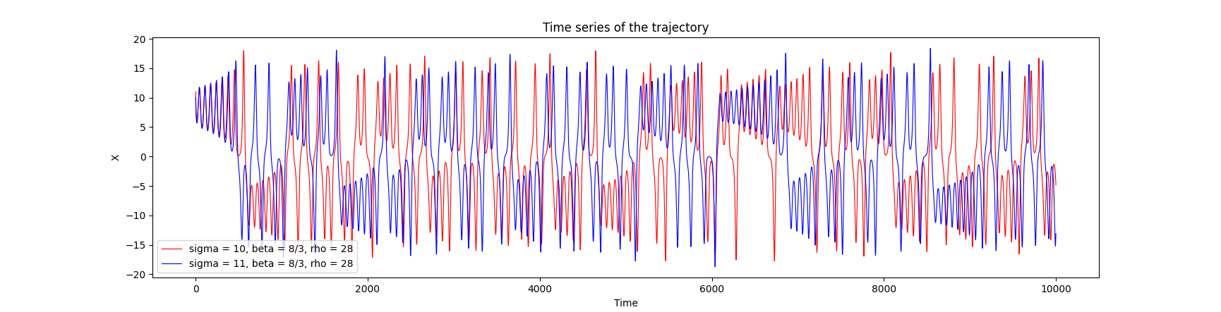
To understand the chaotic behaviour of the lorentz system, two simulations were carried out a different value of sigma. Figure 2 below shows the time series signal of the simulations and it could be visualized that intially the trajectory follow the same path , but later on they start diverging away showing the sensitivity of the system with respect to the intial conditions. Intial condition and Boundray conditioin play a vital role in the behaviour of the system.

As you can see that the with a small change in the initial condition, the output of the system slowly diverges. Lorentz attractor are very sensitive to the intial condition. Figure 3 show the state of lorentz as a function of time, as the system is chaotic it is very difficult to predoi

Animation

To understand the chaotic behavior of the Lorentz system, two simulations were conducted with different values of sigma. In Figure 2, the time series signal of the simulations illustrates that initially, the trajectories follow the same path, but gradually diverge, showcasing the system’s sensitivity to initial conditions. Initial and boundary conditions play a crucial role in determining the system’s behavior.

Indeed, even a slight alteration in the initial condition leads to a gradual divergence in the system’s output. Lorentz attractors exhibit remarkable sensitivity to initial conditions. Figure 3 depicts the state of the Lorentz system over time. Due to its chaotic nature, predicting the behavior becomes exceedingly challenging. The implementation of the lorentz attractor. along with the animation in the corresponding github repository.

Conclusion

The simulations conducted on the Lorentz system vividly demonstrate its chaotic behavior and sensitivity to initial conditions. As showcased in the time series signal and state plots, even minor deviations in initial conditions result in significant divergence in system trajectories. These findings underscore the complexity and unpredictability inherent in chaotic systems like the Lorentz attractor, emphasizing the importance of understanding and carefully managing initial and boundary conditions in modeling and analysis.

Reference

[1] : Lorrentz attractor supporting link.